


Nội dung
Công thức của vấn đề
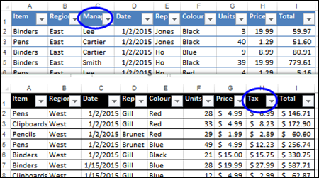
Pivot tables are one of the most amazing tools in Excel. But so far, unfortunately, none of the versions of Excel can do such a simple and necessary thing on the fly as building a summary for several initial data ranges located, for example, on different sheets or in different tables:
Before we start, let’s clarify a couple of points. A priori, I believe that the following conditions are met in our data:
- Tables can have any number of rows with any data, but they must have the same header.
- There should be no extra data on the sheets with source tables. One sheet – one table. To control, I advise you to use a keyboard shortcut Ctrl+Kết thúc, which moves you to the last used cell in the worksheet. Ideally, this should be the last cell in the data table. If when you click on Ctrl+Kết thúc any empty cell to the right or below the table is highlighted – delete these empty columns to the right or rows below the table after the table and save the file.
Method 1: Build tables for a pivot using Power Query
Starting from the 2010 version for Excel, there is a free Power Query add-in that can collect and transform any data and then give it as a source for building a pivot table. Solving our problem with the help of this add-in is not difficult at all.
First, let’s create a new empty file in Excel – assembly will take place in it and then a pivot table will be created in it.
Sau đó trên tab Ngày (nếu bạn có Excel 2016 trở lên) hoặc trên tab Truy vấn nguồn (if you have Excel 2010-2013) select the command Create Query – From File – Excel (Get Data — From file — Excel) and specify the source file with the tables to be collected:

In the window that appears, select any sheet (it doesn’t matter which one) and press the button below Thay đổi (Chỉnh sửa):

The Power Query Query Editor window should open on top of Excel. On the right side of the window on the panel Yêu cầu tham số delete all automatically created steps except the first – nguồn (Nguồn):

Now we see a general list of all sheets. If in addition to data sheets there are some other side sheets in the file, then at this step our task is to select only those sheets from which information needs to be loaded, excluding all the others using the filter in the table header:

Delete all columns except column Ngàyby right-clicking a column heading and selecting Xóa các cột khác (Remove other columns):

You can then expand the contents of the collected tables by clicking on the double arrow at the top of the column (checkbox Sử dụng tên cột ban đầu làm tiền tố you can turn it off):

If you did everything correctly, then at this point you should see the contents of all tables collected one below the other:

It remains to raise the first row to the table header with the button Sử dụng dòng đầu tiên làm tiêu đề (Sử dụng hàng đầu tiên làm tiêu đề) chuyển hướng Trang Chủ (Trang Chủ) and remove duplicate table headers from the data using a filter:

Save everything done with the command Đóng và tải - Đóng và tải vào… (Đóng & Tải - Đóng & Tải vào…) chuyển hướng Trang Chủ (Trang Chủ), and in the window that opens, select the option Chỉ kết nối (Chỉ kết nối):

Everything. It remains only to build a summary. To do this, go to the tab Chèn - PivotTable (Chèn - Bảng tổng hợp), chọn tùy chọn Sử dụng nguồn dữ liệu bên ngoài (Sử dụng nguồn dữ liệu bên ngoài)and then by clicking the button Chọn kết nối, our request. Further creation and configuration of the pivot occurs in a completely standard way by dragging the fields we need into the rows, columns and values area:

If the source data changes in the future or a few more store sheets are added, then it will be enough to update the query and our summary using the command Làm mới tất cả chuyển hướng Ngày (Dữ liệu - Làm mới tất cả).
Method 2. We unite tables with the UNION SQL command in a macro
Another solution to our problem is represented by this macro, which creates a data set (cache) for the pivot table using the command UNITY SQL query language. This command combines tables from all specified in the array SheetNames sheets of the book into a single data table. That is, instead of physically copying and pasting ranges from different sheets to one, we do the same in the computer’s RAM. Then the macro adds a new sheet with the given name (variable ResultSheetName) and creates a full-fledged (!) summary on it based on the collected cache.
To use a macro, use the Visual Basic button on the tab nhà phát triển (Nhà phát triển) hoặc phím tắt Khác+F11. Then we insert a new empty module through the menu Chèn - Mô-đun và sao chép mã sau vào đó:
Sub New_Multi_Table_Pivot() Dim i As Long Dim arSQL() As String Dim objPivotCache As PivotCache Dim objRS As Object Dim ResultSheetName As String Dim SheetsNames As Variant 'sheet name where the resulting pivot will be displayed ResultSheetName = "Pivot" 'an array of sheet names with source tables SheetsNames = Array("Alpha", "Beta", "Gamma", "Delta") 'we form a cache for tables from sheets from SheetsNames With ActiveWorkbook ReDim arSQL(1 To (UBound(SheetsNames) + 1)) For i = LBound (SheetsNames) To UBound(SheetsNames) arSQL(i + 1) = "SELECT * FROM [" & SheetsNames(i) & "$]" Next i Set objRS = CreateObject("ADODB.Recordset") objRS.Open Join$( arSQL, " UNION ALL "), _ Join$(Array("Provider=Microsoft.Jet.OLEDB.4.0; Data Source=", _ .FullName, ";Extended Properties=""Excel 8.0;"""), vbNullString ) End With 're-create the sheet to display the resulting pivot table On Error Resume Next Application.DisplayAlerts = False Worksheets(ResultSheetName).Delete Set wsPivot = Worksheets.Add wsPivot. Name = ResultSheetName 'display the generated cache summary on this sheet Set objPivotCache = ActiveWorkbook.PivotCaches.Add(xlExternal) Set objPivotCache.Recordset = objRS Set objRS = Nothing With wsPivot objPivotCache.CreatePivotTable TableDestination:=wsPivot.Range("A3") Set objPivotCache = Nothing Range("A3").Select End With End Sub The finished macro can then be run with a keyboard shortcut Khác+F8 or the Macros button on the tab nhà phát triển (Nhà phát triển - Macro).
Nhược điểm của cách tiếp cận này:
- The data is not updated because the cache has no connection to the source tables. If you change the source data, you must run the macro again and build the summary again.
- When changing the number of sheets, it is necessary to edit the macro code (array SheetNames).
But in the end we get a real full-fledged pivot table, built on several ranges from different sheets:
Võngà!
Lưu ý kỹ thuật: if you get an error like “Provider not registered” when running the macro, then most likely you have a 64-bit version of Excel or an incomplete version of Office is installed (no Access). To fix the situation, replace the fragment in the macro code:
Provider=Microsoft.Jet.OLEDB.4.0;
đến:
Provider=Microsoft.ACE.OLEDB.12.0;
And download and install the free data processing engine from Access from the Microsoft website – Microsoft Access Database Engine 2010 Redistributable
Method 3: Consolidate PivotTable Wizard from Old Versions of Excel
This method is a little outdated, but still worth mentioning. Formally speaking, in all versions up to and including 2003, there was an option in the PivotTable Wizard to “build a pivot for several consolidation ranges”. However, a report constructed in this way, unfortunately, will only be a pitiful semblance of a real full-fledged summary and does not support many of the “chips” of conventional pivot tables:
In such a pivot, there are no column headings in the field list, there is no flexible structure setting, the set of functions used is limited, and, in general, all this is not very similar to a pivot table. Perhaps that is why, starting in 2007, Microsoft removed this function from the standard dialog when creating pivot table reports. Now this feature is only available through a custom button Trình hướng dẫn PivotTable(Trình hướng dẫn bảng tổng hợp), which, if desired, can be added to the Quick Access Toolbar via File – Options – Customize Quick Access Toolbar – All Commands (File — Options — Customize Quick Access Toolbar — All Commands):

After clicking on the added button, you need to select the appropriate option at the first step of the wizard:

And then in the next window, select each range in turn and add it to the general list:

But, again, this is not a full-fledged summary, so don’t expect too much from it. I can recommend this option only in very simple cases.
- Tạo báo cáo với PivotTables
- Thiết lập tính toán trong PivotTables
- What are macros, how to use them, where to copy VBA code, etc.
- Data collection from multiple sheets to one (PLEX add-on)